(Requires Internet access for the test question) The following question requires you to download data from the internet and to load it into a statistical package such as STATA or EViews.
a. Your textbook suggests using two test statistics to test for stationarity: DF and ADF. Test the null hypothesis that inflation has a stochastic trend against the alternative that it is stationary by performing the DF and ADF test for a unit autoregressive root. That is, use the equation (14.34) in your textbook with four lags and without a lag of the change in the inflation rate as a regressor for sample period 1962:I 2004:IV. Go to the Stock and Watson companion website for the textbook and download the data Macroeconomic Data Used in Chapters 14 and 16. Enter the data for consumer price index, calculate the inflation rate and the acceleration of the inflation rate, and replicate the result on page 526 of your textbook. Make sure not to use the heteroskedasticity-robust standard error option for the estimation.
b. Next find a website with more recent data, such as the Federal Reserve Economic Data (FRED) site at the Federal Reserve Bank of St. Louis. Locate the data for the CPI, which will be monthly, and convert the data in quarterly averages. Then, using a sample from 1962:I 2009:IV, re-estimate the above specification and comment on the changes that have occurred.
c. For the new sample period, find the DF statistic.
d. Finally, calculate the ADF statistic, allowing for the lag length of the inflation acceleration term to be determined by either the AIC or the BIC.
What will be an ideal response?
Question 2
Estimation of dynamic multipliers under strict exogeneity should be done by
A) instrumental variable methods.
B) OLS.
C) feasible GLS.
D) analyzing the stationarity of the multipliers.

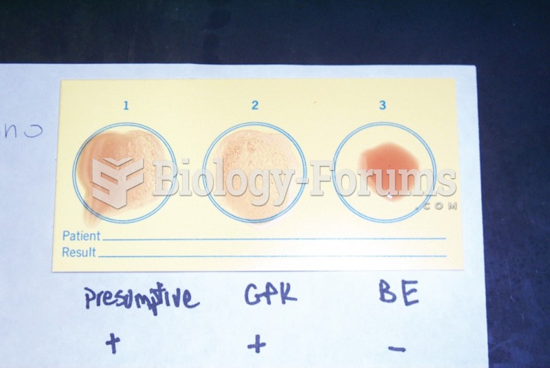 A Mono-Diff test in which the presumptive well contains the patient's serum mixed with ...
 Water Access
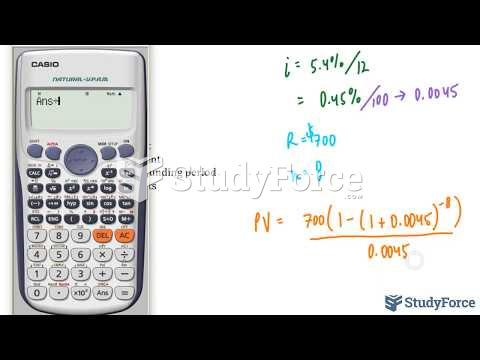 How to calculate present value (Question 1)
 How to create a table of values displaying commission and earnings (Question 1)
 this is a math question
 economic question