Answer to Question 1
When timelines are used as evidence, it is necessary that they be reliable. Of course, the reliability of a timeline depends on the reliability of its components-the timing of individual events. Although time is an objective measure, this does not mean that all measurements of time are reliable. As with all forms of data, a primary factor in assessing reliability is the source. Time can be obtained from any device that has a clock, which includes most computerized devices (such as personal computers, cell phones, cash registers, and ATMs). Investigators can also obtain timing information from other documents. For example, checks are dated, receipts are time-stamped, and computers record the time a file was created, accessed, and modified. The investigator must be aware that, while time is objective, the measurement of time is vulnerable to human manipulation and error. Computer clocks can be adjusted, power failures can produce inaccuracies, and people can misdate documents, either intentionally or unintentionally. Thus, it is important to assess the validity of time measurements before relying on them.
Answer to Question 2
1. Mandy will pick the highest point of activity, 4,068 parts (March) at 17,280 of cost, and the lowest point of activity, 2,316 parts (August) at 10,272.
Cost driver:
Quantity Purchased Cost
Highest observation of cost driver 4,068 17,280
Lowest observation of cost driver 2,316 10,272
Difference 1,752 7,008
Purchase costs = a + b Quantity purchased
Slope Coefficient = 7,008/1,752 = 4 per part
Constant (a) = 17,280 (4 4,068) = 1,008
The equation Mandy gets is:
Purchase costs = 1,008 + (4 Quantity purchased)
2. Using the equation above, the expected purchase costs for each month will be:
Month Purchase Quantity
Expected Formula Expected
cost
October 3,360 parts y = 1,008 + (4 3,360) 14,448
November 3,720 y = 1,008 + (4 3,720) 15,888
December 3,000 y = 1,008 + (4 3,000) 13,008
3. Economic Plausibility: Clearly, the cost of purchasing a part is associated with the quantity purchased.
Goodness of Fit: As seen in Solution Exhibit 10- 27, the regression line fits the data well. The vertical distance between the regression line and observations is small. An r-squared value of greater than 0.98 indicates that more than 98 percent of the change in cost can be explained by the change in quantity.
Significance of the Independent Variable: The relatively steep slope of the regression line suggests that the quantity purchased is correlated with purchasing cost for part 696.
EXHIBIT 10- 27
According to the regression, Mandy's original estimate of fixed cost is too low given all the data points. The original slope is too steep but only by 33 cents. So, the variable rate is lower, but the fixed cost is higher for the regression line than for the high-low cost equation.
The regression is the more accurate estimate because it uses all available data (all nine data points), while the high-low method only relies on two data points and may therefore miss some important information contained in the other data.
4. Using the regression equation, the purchase costs for each month will be:
Month Purchase
Quantity
Expected Formula Expected cost
October 3,360 parts y = 2,135.50 + (3.67 3,360) 14,466.70
November 3,720 y = 2,135.50 + (3.67 3,720) 15,787.90
December 3,000 y = 2,135.50 + (3.67 3,000) 13,145.50
Although the two equations are different in both fixed element and variable rate, within the relevant range they give similar expected costs. This implies that the high and low points of the data are a reasonable representation of the total set of points within the relevant range.


